Statistics > Normal Distribution
The Normal Distribution
(Bell Curve)
In many natural processes, random variation conforms to a particular probability distribution known as the normal distribution, which is the most commonly observed probability distribution. Mathematicians de Moivre and Laplace used this distribution in the 1700's. In the early 1800's, German mathematician and physicist Karl Gauss used it to analyze astronomical data, and it consequently became known as the Gaussian distribution among the scientific community.
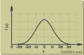
The shape of the normal distribution resembles that of a bell, so it sometimes is referred to as the "bell curve", an example of which follows:
Normal Distribution

The above curve is for a data set having a mean of zero. In general, the normal distribution curve is described by the following probability density function:
Bell Curve Characteristics
The bells curve has the following characteristics:
- Symmetric
- Unimodal
- Extends to +/- infinity
- Area under the curve = 1
Completely Described by Two Parameters
The normal distribution can be completely specified by two parameters:
- mean
- standard deviation
If the mean and standard deviation are known, then one essentially knows as much as if one had access to every point in the data set.
The Empirical Rule
The empirical rule is a handy quick estimate of the spread of the data given the mean and standard deviation of a data set that follows the normal distribution.
The empirical rule states that for a normal distribution:
- 68% of the data will fall within 1 standard deviation of the mean
- 95% of the data will fall within 2 standard deviations of the mean
- Almost all (99.7%) of the data will fall within 3 standard deviations of the mean
Note that these values are approximations. For example, according to the normal curve probability density function, 95% of the data will fall within 1.96 standard deviations of the mean; 2 standard deviations is a convenient approximation.
Normal Distribution and the Central Limit Theorem
The normal distribution is a widely observed distribution. Furthermore, it frequently can be applied to situations in which the data is distributed very differently. This extended applicability is possible because of the central limit theorem, which states that regardless of the distribution of the population, the distribution of the means of random samples approaches a normal distribution for a large sample size.
Applications to Business Administration
The normal distribution has applications in many areas of business administration. For example:
- Modern portfolio theory commonly assumes that the returns of a diversified asset portfolio follow a normal distribution.
- In operations management, process variations often are normally distributed.
- In human resource management, employee performance sometimes is considered to be normally distributed.
The normal distribution often is used to describe random variables, especially those having symmetrical, unimodal distributions. In many cases however, the normal distribution is only a rough approximation of the actual distribution. For example, the physical length of a component cannot be negative, but the normal distribution extends indefinitely in both the positive and negative directions. Nonetheless, the resulting errors may be negligible or within acceptable limits, allowing one to solve problems with sufficient accuracy by assuming a normal distribution.
Statistics > Normal Distribution


